

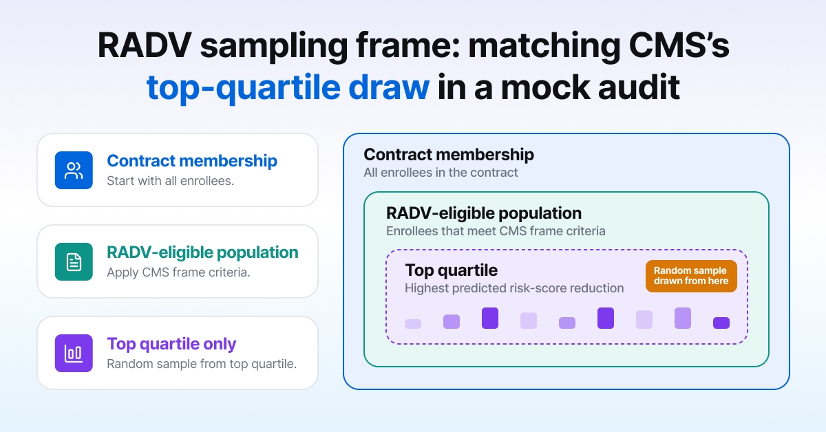
A RADV sampling frame is the set of enrollees CMS draws from when it selects a contract’s audit sample, and for PY2024 it is the enrollees CMS’s own improper-payment prediction models rank in the top quartile for expected risk-score reduction. The random draw happens inside that quartile. A mock audit that samples 35 members at random from the full membership measures a different population from the one CMS will audit, which is the point of the prediction model.
Eight frame conditions, one of which does the work
Section 4.1 of the PY2024 methods and instructions defines the frame. An enrollee is in it if they:
- were continuously enrolled in the contract from January 2023 through January 2024;
- had twelve months of Part B in 2023;
- had at least one 2023 diagnosis that produced an HCC for PY2024;
- were not in ESRD status;
- were not in hospice status;
- were not part of an OIG audit or settlement covering the period;
- were not enrolled in a C-SNP, I-SNP, or FIDE-SNP; and
- were ranked in the top quartile of RADV-eligible enrollees across all contracts, an expansion from the top decile used in the PY2018 and PY2019 audits, by one or both of CMS’s PY2024 improper-payment prediction models, “and, therefore, predicted to have the greatest reduction in their risk score as a result of a RADV audit.”
Within that frame, CMS draws a simple random sample without replacement, seeded and selected in SAS:
| Stratum | Contracts | Sample size |
|---|---|---|
| 1 | Ten largest sampling frames | 200 |
| 2 | Top third of the rest | 100 |
| 3 | Middle third | 50 |
| 4 | Bottom third | 35 |
If the frame is smaller than the stratum’s sample size, every enrollee in it is audited.
What this means. The sample is random and the population is not. The expected error rate in a CMS sample is higher than the contract-wide rate by construction, so any internal estimate that ignores the quartile filter is optimistic. And the frame is a signal about which enrollees CMS thinks are weak, most of which a plan can reproduce from public information.
Proxy ranker: the public signals that predict a risk-score drop
CMS has not published the prediction models. It has published what it audits, what it finds, and what it excludes, and that is enough to build a proxy that ranks enrollees the same way for most of the distribution. The strongest features are the ones OIG has reported for years:
- an HCC resting on a single encounter in the year, especially a health risk assessment or a chart-review record rather than a treating visit;
- codes in OIG’s high-risk groups, which are acute stroke, acute MI, embolism, and the four named cancers, plus patterns from OIG’s contract-level audits such as major depression with no severity;
- high-coefficient HCCs generally, because a discrepancy there produces a larger risk-score drop, which is what the model is trained to predict;
- diagnoses whose only source is a problem list;
- provider-type anomalies, such as a specialist diagnosis with no matching specialty in the encounter.
A proxy model built on those features and trained on your own historical mock-audit outcomes will not reproduce CMS’s ranking exactly. It does not have to. It has to put the same enrollees in the top quartile often enough that the internal sample looks like the CMS sample, and in our experience a gradient-boosted ranker over those features gets most of the way there. The residual disagreement is worth studying, because it tells you which of your weak enrollees CMS may not see, and which of CMS’s targets you are not looking at. The HCC coding gaps explainer covers the source-of-diagnosis features from the capture side.
Extrapolation math: the 90% lower bound decides
Section 9.2 describes how CMS would extrapolate if it collects extrapolated amounts, and the RADV Hub has a worked example. The mock audit has to reproduce it to be useful.
- For each sampled enrollee, compute the change in risk score (original minus post-audit), weighted by enrollment months if the enrollee was not enrolled all year.
- Average those changes across the sample. That is the point estimate.
- Compute the sample variance with a finite-population correction, (N − n)/N, where N is the frame and n the sample.
- Take the lower bound of a 90% confidence interval, using a t-statistic with n − 1 degrees of freedom.
- If that lower bound is above zero, the extrapolated payment error is the average change in risk score multiplied by the sum of county rates across every enrollee in the frame. If it is at or below zero, CMS collects only the sampled-enrollee amounts.
Extrapolation is also off when the sampling frame has fewer than 30 enrollees and CMS is auditing all HCCs, in which case CMS audits the entire frame. Underpayments are capped at zero at the contract level, and additional HCCs found during abstraction offset overpayments only when they sit in the same hierarchy as an audited HCC. A note that supports a higher-severity code than was submitted helps. A note that supports an unrelated HCC nobody submitted does not.
Two properties of this calculation surprise finance teams. A 35-enrollee sample with a few large discrepancies and many zeros has high variance, a wide interval, and a lower bound that often crosses zero, so a small contract can escape extrapolation with the same mean error that would trigger it at 200. And the multiplier is the frame’s total county rates, so the exposure scales with the high-risk quartile’s payments, not with membership.
Sampler design: four stages, several hundred draws
The design I would build, and the one we built, has four stages:
- Frame. Apply the eight conditions to the contract’s membership as of the data collection year.
- Rank. Score each eligible enrollee with the proxy ranker and keep the top quartile.
- Draw. Select the stratum sample size at random from that quartile, with a stored seed so the draw is reproducible.
- Validate and compute. Check every audited HCC for the sampled enrollees against MEAT criteria and the CMS record rules, compute the change in risk score under the payment year’s model (blended for PY2024), and run the section 9.2 calculation to produce sample-only exposure and extrapolated exposure with its confidence bound.
Then repeat stages 3 and 4 several hundred times with different seeds. The distribution of extrapolated exposure across draws tells you how sensitive the contract is to which 35 or 200 enrollees CMS happens to pick, which is a better answer for a CFO than a single point estimate. It also tells you where the variance comes from, enrollee by enrollee, which is the prioritized fix list.
“35 random members” is a QA exercise, not a mock audit
“We sampled 35 random members last year and validated 92% of the HCCs.” That sentence describes the contract-wide population, not the frame CMS audits. It says nothing about the top quartile, where OIG’s plan-level audits (listed on the RADV Hub) found about 70% of sampled high-risk codes unsupported, and certain code groups over 90%. It also gives no confidence interval, so it cannot say whether the 8% failure rate would extrapolate. A mock audit that cannot answer both questions is a coding QA exercise, which is a fine thing to have and a different thing from RADV readiness.
Martlet AI’s mock RADV samples from a reconstructed frame, validates each sampled HCC with page-level evidence, and reports sample-only and extrapolated exposure per contract with the confidence bound, all inside the plan’s environment. If you have a contract in the PY2023 cycle that initiates this month, run it through a mock audit before the enrollee data list arrives and compare the two samples.
FAQ
Does CMS select RADV enrollees at random?
The draw is random, but the population it draws from is not. For PY2024, the sampling frame is limited to enrollees ranked in the top quartile by CMS’s improper-payment prediction models, after excluding ESRD, hospice, certain SNP enrollees, and enrollees covered by OIG audits.
Has CMS published its improper-payment prediction models?
No. The methods document describes their purpose (predicting the greatest reduction in risk score from a RADV audit) but not their features or weights. A plan can approximate the ranking from OIG’s published high-risk patterns and its own mock-audit history.
How does CMS decide whether to extrapolate?
It computes the average change in risk score across the sample and the lower bound of a 90% confidence interval on that average. If the lower bound is above zero, the average is multiplied by the sum of county rates for the whole frame. Extrapolation is not used when the frame has fewer than 30 enrollees and CMS is auditing all HCCs, and as of PY2024 CMS collects sampled-enrollee amounts only while the 2023 rule is on appeal.
Why can a 35-enrollee sample escape extrapolation when a 200-enrollee sample does not?
Smaller samples have higher variance, which widens the confidence interval. With the same average error, a 35-enrollee sample’s lower bound is more likely to cross zero.
Do additional HCCs found in the audit reduce the overpayment?
Only when they are in the same hierarchy as an audited HCC. Unrelated HCCs found during abstraction do not offset, and no RADV audit results in additional payment to the plan.
What should a mock RADV report?
Sample-only exposure, extrapolated exposure with the 90% lower bound, the distribution of both across repeated draws, and a per-enrollee list of the HCCs driving the variance, so the fix list is prioritized.